
11 KiB
| layout | title |
|---|---|
| post | Outbreak Detection in Networks |
Introduction
The general goal of outbreak detection in networks is that given a dynamic process spreading over a network, we want to select a set of nodes to detect the process efficiently. Outbreak detection in networks has many applications in real life. For example, where should we place sensors to quickly detect contaminations in a water distribution network? Which person should we follow on Twitter to avoid missing important stories?
The following figure shows the different effects of placing sensors at two different locations in a network:
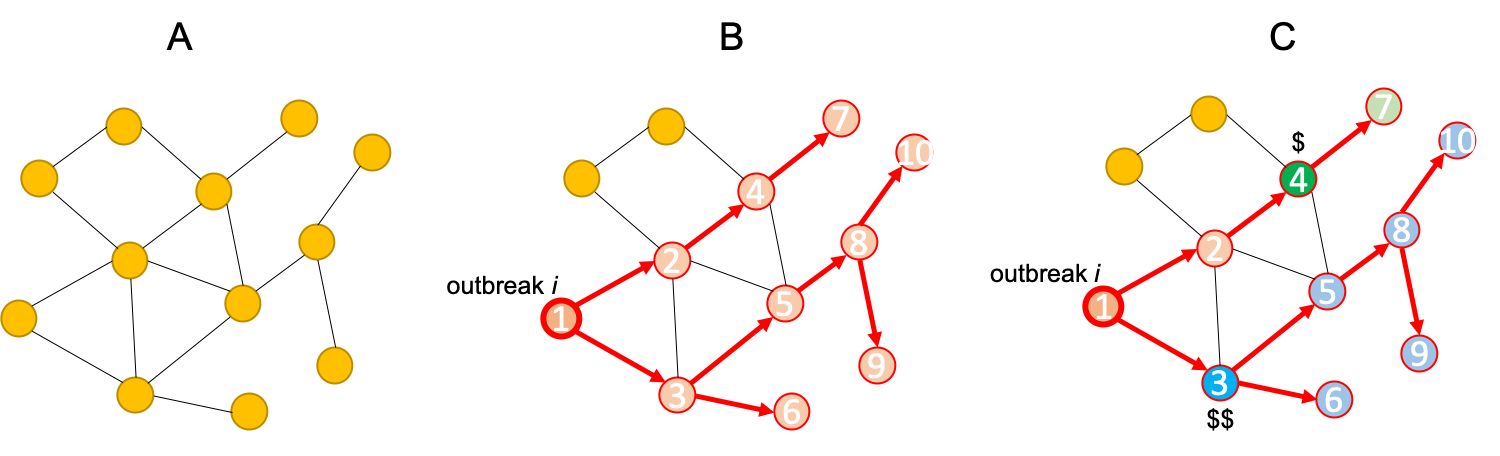 (A) The given network. (B) An outbreak $$i$$ starts and spreads as shown. (C) Placing a sensor at the blue position saves more people and also detects earlier than placing a sensor at the green position, though costs more.
Problem Setup
The outbreak detection problem is defined as below:
- Given: a graph $$G(V,E)$$ and data on how outbreaks spread over this $$G$$ (for each outbreak $$i$$, we knew the time $$T(u,i)$$ when the outbreak $$i$$ contaminates node $$u$$).
- Goal: select a subset of nodes $$S$$ that maximize the expected reward:
$$ \max_{S\subseteq U}f(S)=\sum_{i}p(i)\cdot f_{i}(S) $$
$$ \text{subject to cost }c(S)\leq B $$
where
- $$p(i)$$: probability of outbreak $$i$$ occurring
- $$f_{i}(S)$$: rewarding for detecting outbreak $$i$$ using "sensors" $$S$${% include sidenote.html id='note-outbreak-detection-problem-setup' note='It is obvious that $$p(i)\cdot f_{i}(S)$$ is the expected reward for detecting the outbreak $$i$$' %}
- $$B$$: total budget of placing "sensors"
The Reward can be one of the following three:
- Minimize the time to detection
- Maximize the number of detected propagations
- Minimize the number of infected people
The Cost is context-dependent. Examples are:
- Reading big blogs is more time consuming
- Placing a sensor in a remote location is more expensive
Outbreak Detection Formalization
Objective Function for Sensor Placements
Define the **penalty $$\pi_{i}(t)$$** for detecting outbreak $$i$$ at time $$t$$, which can be one of the following:{% include sidenote.html id='note-outbreak-detection-penalty-note' note='Notice: in all the three cases detecting sooner does not hurt! Formally, this means, for all three cases, $$\pi_{i}(t)$$ is monotonically nondecreasing in $$t$$.'%}
-
Time to Detection (DT)
- How long does it take to detect an outbreak?
- Penalty for detecting at time $$t$$: $$\pi_{i}(t)=t$$
-
Detection Likelihood (DL)
- How many outbreaks do we detect?
- Penalty for detecting at time $$t$$: $$\pi_{i}(0)=0$$, $$\pi_{i}(\infty)=1$${% include sidenote.html id='note-penalty-dl' note='this is a binary outcome: $$\pi_{i}(0)=0$$ means we detect the outbreak and we pay 0 penalty, while $$\pi_{i}(\infty)=1$$ means we fail to detect the outbreak and we pay 1 penalty. That is we do not incur any penalty if we detect the outbreak in finite time, otherwise we incur penalty 1.'%}
-
Population Affected (PA)
- How many people/nodes get infected during an outbreak?
- Penalty for detecting at time $$t$$: $$\pi_{i}(t)=$$ number of infected nodes in the outbreak $$i$$ by time $$t$$
The objective **reward function $$f_{i}(S)$$ of a sensor placement $$S$$** is defined as penalty reduction:
$$ f_{i}(S)=\pi_{i}(\infty)-\pi_{i}(T(S,i)) $$
where $$T(S,i)$$ is the time when the set of "sensors" $$S$$ detects the outbreak $$i$$.
Claim 1: $$f(S)=\sum_{i}p(i)\cdot f_{i}(S)$$ is monotone{% include sidenote.html id='note-monotone' note='For the definition of monotone, see Influence Maximization' %}
Firstly, we do not reduce the penalty, if we do not place any sensors. Therefore, $$f_{i}(\emptyset)=0$$ and $$f(\emptyset)=\sum_{i}p(i)\cdot f_{i}(\emptyset)=0$$.
Secondly, for all $$A\subseteq B\subseteq V$$ ($$V$$ is all the nodes in $$G$$), $$T(A,i)\geq T(B,i)$$, and
$$
\begin{align*}
f_{i}(A)-f_{i}(B)&=\pi_{i}(\infty)-\pi_{i}(T(A,i))-[\pi_{i}(\infty)-\pi_{i}(T(B,i))]\
&=\pi_{i}(T(B,i))-\pi_{i}(T(A,i))
\end{align*}
$$
Because $$\pi_{i}(t)$$ is monotonically nondecreasing in $$t$$ (see sidenote 2), $$f_{i}(A)-f_{i}(B)<0$$. Therefore, $$f_{i}(S)$$ is nondecreasing. It is obvious that $$f(S)=\sum_{i}p(i)\cdot f_{i}(S)$$ is also nondecreasing, since $$p(i)\geq 0$$.
Hence, $$f(S)=\sum_{i}p(i)\cdot f_{i}(S)$$ is monotone.
Claim 2: $$f(S)=\sum_{i}p(i)\cdot f_{i}(S)$$ is submodular{% include sidenote.html id='note-submodular' note='For the definition of submodular, see Influence Maximization' %}
This is to proof for all $$A\subseteq B\subseteq V$$ $$x\in V \setminus B$$:
$$ f(A\cup {x})-f(A)\geq f(B\cup{x})-f(B) $$
There are three cases when sensor $$x$$ detects the outbreak $$i$$:
- $$T(B,i)\leq T(A, i)<T(x,i)$$ ($$x$$ detects late): nobody benefits. That is $$f_{i}(A\cup{x})=f_{i}(A)$$ and $$f_{i}(B\cup{x})=f_{i}(B)$$. Therefore, $$f(A\cup {x})-f(A)=0= f(B\cup{x})-f(B)$$
- $$T(B, i)\leq T(x, i)<T(A,i)$$ ($$x$$ detects after $$B$$ but before $$A$$): $$x$$ only helps to improve the solution of $$A$$ but not $$B$$. Therefore, $$f(A\cup {x})-f(A)\geq 0 = f(B\cup{x})-f(B)$$
- $$T(x, i)<T(B,i)\leq T(A,i)$$ ($$x$$ detects early): $$f(A\cup {x})-f(A)=[\pi_{i}(\infty)-\pi_{i}(T(x,t))]-f_{i}(A)$$$$ \geq [\pi_{i}(\infty)-\pi_{i}(T(x,t))]-f_{i}(B) = f(B\cup{x})-f(B)$${% include sidenote.html id='note-submodularity-proof1' note='Inequality is due to the nondecreasingness of $$f_{i}(\cdot)$$, i.e. $$f_{i}(A)\leq f_{i}(B)$$ (see Claim 1).'%}
Therefore, $$f_{i}(S)$$ is submodular. Because $$p(i)\geq 0$$, $$f(S)=\sum_{i}p(i)\cdot f_{i}(S)$$ is also submodular.{% include sidenote.html id='note-submodularity-proof1' note='Fact: a non-negative linear combination of submodular functions is a submodular function.'%}
We know that the Hill Climbing algorithm works for optimizing problems with nondecreasing submodular objectives. However, it does not work well in this problem:
- Hill Climbing only works for the cases that each sensor costs the same. For this problem, each sensor has cost $$c(s)$$.
- Hill Climbing is also slow: at each iteration, we need to re-evaluate marginal gains of all nodes. The run time is $$O(\mid V\mid\cdot k)$$ for placing $$k$$ sensors.
Hence, we need a new fast algorithm that can handle cost constraints.
CELF: Algorithm for Optimziating Submodular Functions Under Cost Constraints
Bad Algorithm 1: Hill Climbing that ignores the cost
Algorithm
- Ignore sensor cost $$c(s)$$
- Repeatedly select sensor with highest marginal gain
- Do this until the budget is exhausted
This can fail arbitrarily bad! Example:
- Given $$n$$ sensors and a budget $$B$$
- $$s_{1}$$: reward $$r$$, cost $$B$$
- $$s_{2}$$,..., $$s_{n}$$: reward $$r-\epsilon$$, cost $$\epsilon$$ ($$\epsilon$$ is an arbitrary positive small number)
- Hill Climbing always prefers $$s_{1}$$ to other cheaper sensors, resulting in an arbitrarily bad solution with reward $$r$$ instead of the optimal solution with reward $$\frac{B(r-\epsilon)}{\epsilon}$$, when $$\epsilon \rightarrow 0$$.
Bad Algorithm 2: optimization using benefit-cost ratio
Algorithm
- Greedily pick the sensor $$s_{i}$$ that maximizes the benefit to cost ratio until the budget runs out, i.e. always pick
$$ s_{i}=\arg\max_{s\in(V\setminus A_{i-1})}\frac{f(A_{i-1}\cup{s})-f(A_{i-1})}{c(s)} $$
This can fail arbitrarily bad! Example:
- Given 2 sensors and a budget $$B$$
- $$s_{1}$$: reward $$2\epsilon$$, cost $$\epsilon$$
- $$s_{2}$$: reward $$B$$, cost $$B$$
- Then the benefit ratios for the first selection are: 2 and 1, respectively
- This algorithm will pick $$s_{1}$$ and then cannot afford $$s_{2}$$, resulting in an arbitrarily bad solution with reward $$2\epsilon$$ instead of the optimal solution $$B$$, when $$\epsilon \rightarrow 0$$.
Solution: CELF (Cost-Effective Lazy Forward-selection)
CELF is a two-pass greedy algorithm [Leskovec et al. 2007]:
- Get solution $$S'$$ using unit-cost greedy (Bad Algorithm 1)
- Get solution $$S''$$ using benefit-cost greedy (Bad Algorithm 2)
- Final solution $$S=\arg\max[f(S'), f(S'')]$$
Approximation Guarantee
- CELF achieves $$\frac{1}{2}(1-\frac{1}{e})$$ factor approximation.
CELF also uses a lazy evaluation of $$f(S)$$ (see below) to speedup Hill Climbing.
Lazy Hill Climbing: Speedup Hill Climbing
Intuition
- In Hill Climbing, in round $$i+1$$, we have picked $$S_{i}={S_{1},...,S_{i}}$$ sensors. Now, pick $$s_{i+1}=\arg\max_{u}f(S_{i}\cup {u})-f(S_{i})$$
- By submodularity $$f(S_{i}\cup{u})-f(S_{i})\geq f(S_{j}\cup{u})-f(S_{j})$$ for $$i<j$$.
- Let $$\delta_{i}(u)=f(S_{i}\cup{u})-f(S_{i})$$ and $$\delta_{j}(u)=f(S_{j}\cup{u})-f(S_{j})$$ be the marginal gains. Then, we can use $$\delta_{i}$$ as upper bound on $$\delta_{j}$$ for ($$j>i$$)
Lazy Hill Climbing Algorithm:
- Keep an ordered list of marginal benefits $$\delta_{i-1}$$ from previous iteration
- Re-evaluate $$\delta_{i}$$ only for the top nodes
- Reorder and prune from the top nodes
The following figure show the process.
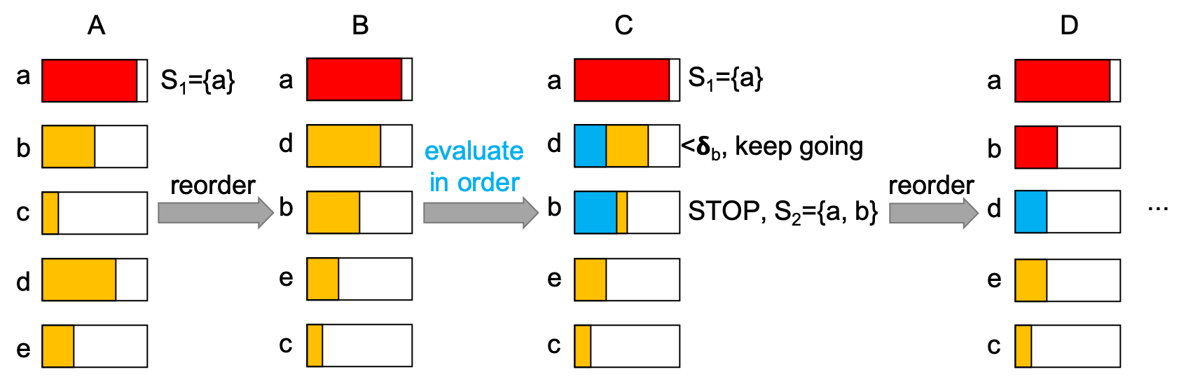
(A) Evaluate and pick the node with the largest marginal gain $$\delta$$. (B) reorder the marginal gain for each sensor in decreasing order. (C) Re-evaluate the $$\delta$$s in order and pick the possible best one by using previous $$\delta$$s as upper bounds. (D) Reorder and repeat.
Note: the worst case of Lazy Hill Climbing has the same time complexity as normal Hill Climbing. However, it is on average much faster in practice.
Data-Dependent Bound on the Solution Quality
Introduction
- Value of the bound depends on the input data
- On "easy data", Hill Climbing may do better than the $$(1-\frac{1}{e})$$ bound for submodular functions
Data-Dependent Bound
Suppose $$S$$ is some solution to $$f(S)$$ subjected to $$\mid S \mid\leq k$$, and $$f(S)$$ is monotone and submodular.
- Let $$OPT={t_{i},...,t_{k}}$$ be the optimal solution
- For each $$u$$ let $$\delta(u)=f(S\cup{u})-f(S)$$
- Order $$\delta(u)$$ so that $$\delta(1)\geq \delta(2)\geq...$$
- Then, the data-dependent bound is $$f(OPT)\leq f(S)+\sum^{k}_{i=1}\delta(i)$$
Proof:{% include sidenote.html id='note-data-dependent-bound-proof' note='For the first inequality, see the lemma in 3.4.1 of this handout. For the last inequality in the proof: instead of taking $$t_{i}\in OPT$$ of benefit $$\delta(t_{i})$$, we take the best possible element $$\delta(i)$$, because we do not know $$t_{i}$$.'%}
$$
\begin{align*}
f(OPT)&\leq f(OPT\cup S)\
&=f(S)+f(OPT\cup S)-f(S)\
&\leq f(S)+\sum^{k}_{i=1}[f(S\cup{t_{i}})-f(S)]\
&=f(S)+\sum^{k}_{i=1}\delta(t_{i})\
&\leq f(S)+\sum^{k}_{i=1}\delta(i)
\end{align*}
$$
Note:
- This bound hold for the solution $$S$$ (subjected to $$\mid S \mid\leq k$$) of any algorithm having the objective function $$f(S)$$ monotone and submodular.
- The bound is data-dependent, and for some inputs it can be very "loose" (worse than $$(1-\frac{1}{e})$$)