5.4 KiB
Motifs and Structral Rules in Network
Subgraphs
In this section, we will begin by introducing the defination of subgraphs. Subnetworks, or subgraphs, are the building blocks of networks which enable us to characterize and discriminate networks.
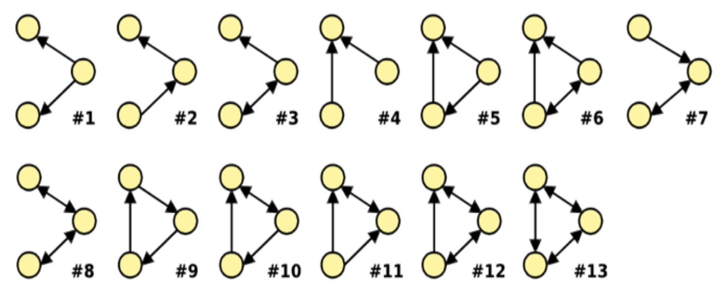
For example, in Figure 1 we show all the non-isomorphic directed subgraphs of size 3. These subgraphs differ from each other in the number of edges or direction of edges.
Motifs
Network motifs are recurring, significant patterns of interconnections in the network. Here, pattern means it is small induced subgraph. Note induced subgraph of graph G is a graph formed from a subset X of the vertices of graph G and all of the edges connecting pairs of vertices in subset X.
Recurrence of motif represents it occurs with high frequency. We allow overlapping of motifs.
Significance of a motif means it is more frequent than expected. The key idea here is we say subgraphs that occur in a real network much more often than in a random network have functional significance. Significance can be measured using Z-score which is defined as: \begin{equation} Z_{i} = \frac{N_{i}^{real} - \overline N_{i}^{rand}}{std(N_{i}^{rand})} \end{equation}
where $N_{i}^{real}$ is #(subgraphs of type i) in network $G^{real}$ and $N_{i}^{rand}$ is #(subgraphs of type i) in randomized network $G^{rand}$.
Network significance profile (SP) is defined as: \begin{equation} SP_{i} = \frac{Z_{i}}{\sqrt{\sum_{j} {Z_j^{2}}}} \end{equation} where SP is a vector of normalized Z-scores.
Configuration Model
Configuration model is a random graph with a given degree sequence $k_1$, $k_2$, ..., $k_N$ which can be used as a "null" model and then compared with real network. Configuration model can be generated in an easy way as shown in Figure 2.
Another way for generation is as following:
- start from a given graph G;
- select a pair of edges A->B, C->D at random, exchange the endpoints to give A->D, C->B, repeat the switching step Q* \vert E \vert times.
By this way, we will get a randomly rewired graph with same node degrees and randomly rewired edges.
Graphlets
Graphlets are connected non-isomorphic subgraphs. It allows us to obtain a node-level subgraph metric. Graphlet Degree Vector (GDV) is a vector with the frequency of the node in each orbit position, it counts the number of graphlets that a node touches. GDV provides a measure of a node's local network topology.
Finding Motifs and Graphlets
Finding size-k motifs/graphlets requires us:
- enumerate all size-k connected subgraphs;
- count the number of occurrences of each subgraph type.
Just knowing if a certain subgraph exists in a graph is a hard computational problem. Also, computation time grows exponentially as the size of the motif/graphlet increases.
ESU Algorithm
Exact Subgraph Enumeration (ESU) Algorithm involves two sets, while $V_{subgraph}$ contains nodes in currently constructed subgraph, and $V_{extension}$ is a set of candidate nodes to extend the motif. The basic idea of ESU is firstly starting with a node v, then adding nodes u to $V_{extension}$ set when u's node id is larger than that of v, and u may only be neighbored to some newly added node w but not of any node already in $V_{subgraph}$.
ESU is implemented as a recursive function, Figure 3 shows the pseudocode of this algorithm: ** Figure**
Structural Roles in Networks
Roles
We can consider roles as functions of nodes in a network which can be measured by structural behaviors. Note roles are different from groups/communities. Roles are based on the similarity of ties between subsets of nodes. Nodes with the same role have similar structural properties, but they don't need to be in direct or even indirect interaction with each other. Group/community is formed based on adjacency, proximity or reachability, nodes in the same community are well-connected to each other.
Structural equivalence
We say nodes u and v are structurally equivalent if they have the same relationships to each other. Structurally equivalent nodes are likely to be similar in many different ways. For example, node u and v are structurally equivalent in Figure # since they connect other nodes in the same way.
RoIX
Roles allow us to identify different properties of nodes in network. Here we will introduce an automatic structural roles discovery method called RolX. It's an unsupervised learning approach without prior knowledge. Figure 5 is the RoIX approach overview.
Recursive Feature Extraction
The basic idea of recursive feature extraction is to aggregate features of a node and use them to generate new recursive features. By this way we can turn network connectivity into structural features.
The base set of a node's neighborhood features include:
- Local features, which are all measures of the node degree.
- Egonet features, which are computed on the node's egonet and may include the number of within-egonet edges, and the number of edges entering/leaving egonet. Here egonet of a node includes the node itself, its neighbors and any edges in the induced subgraph on these nodes.
To generate recursive features, firstly we start with the base set of node features, then use the set of current node features to generate additional features and repeat. The number of possible recursive features grows exponentially with each recursive iteration.


