
11 KiB
| layout | title |
|---|---|
| post | Influence Maximization |
Motivation
Identification of influential nodes in a network has important practical uses. A good example is "viral marketing", a strategy that uses existing social networks to spread and promote a product. A well-engineered viral marking compaign will identify the most influential customers, convince them to adopt and endorse the product, and then spread the product in the social network like a virus.
The key question is how to find the most influential set of nodes? To answer this question, we will first look at two classical cascade models:
- Linear Threshold Model
- Independent Cascade Model
Then, we will develop a method to find the most influential node set in the Independent Cascade Model.
Linear Threshold Model
In the Linear Threshold Model, we have the following setup:
- A node $$v$$ has a random threshold $$\theta_{v} \sim U[0,1]$$
- A node $$v$$ influenced by each neighbor $$w$$ according to a weight $$b_{v,w}$$, such that
$$ \sum_{w\text{ neighbor of v }} b_{v,w}\leq 1 $$
- A node $$v$$ becomes active when at least $$\theta_{v}$$ fraction of its neighbors are active. That is
$$ \sum_{w\text{ active neighbor of v }} b_{v,w}\geq\theta_{v} $$
The following figure demonstrates the process:
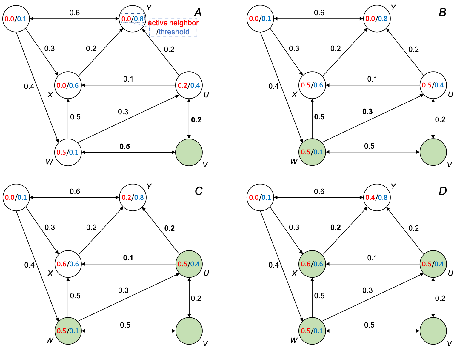
(A) node V is activated and influences W and U by 0.5 and 0.2, respectively; (B) W becomes activated and influences X and U by 0.5 and 0.3, respectively; (C) U becomes activated and influences X and Y by 0.1 and 0.2, respectively; (D) X becomes activated and influences Y by 0.2; no more nodes can be activated; process stops.
Independent Cascade Model
In this model, we model the influences (activation) of nodes based on probabilities in a directed graph:
- Given a directed finite graph $$G=(V, E)$$
- Given a node set $$S$$ starts with a new behavior (e.g. adopted new product and we say they are active)
- Each edge $$(v, w)$$ has a probability $$p_{vw}$$
- If node $$v$$ becomes active, it gets one chance to make $$w$$ active with probability $$p_{vw}$$
- Activation spread through the network
Note:
- Each edge fires only once
- If $$u$$ and $$v$$ are both active and link to $$w$$, it does not matter which tries to activate $$w$$ first
Influential Maximization (of the Independent Cascade Model)
Definitions
- Most influential Set of size $$k$$ ($$k$$ is a user-defined parameter) is a set $$S$$ containing $$k$$ nodes that if activated, produces the largest expected{% include sidenote.html id='note-most-influential-set' note='Why "expected cascade size"? Due to the stochastic nature of the Independent Cascade Model, node activation is a random process, and therefore, $$f(S)$$ is a random variable. In practice, we would like to compute many random simulations and then obtain the expected value $$f(S)=\frac{1}{\mid I\mid}\sum_{i\in I}f_{i}(S)$$, where $$I$$ is a set of simulations.' %} cascade size $$f(S)$$.
- **Influence set $$X_{u}$$ of node $$u$$** is the set of nodes that will be eventually activated by node $$u$$. An example is shown below.
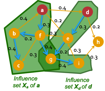
*Red-colored nodes a and b are active. The two green areas enclose the nodes activated by a and b respectively, i.e. $$X_{a}$$ and $$X_{b}$$.*
Note:
- It is clear that $$f(S)$$ is the size of the union of $$X_{u}$$: $$f(S)=\mid\cup_{u\in S}X_{u}\mid$$.
- Set $$S$$ is more influential, if $$f(S)$$ is larger
Problem Setup
The influential maximization problem is then an optimization problem:
$$ \max_{S \text{ of size }k}f(S) $$
This problem is NP-hard [Kempe et al. 2003]. However, there is a greedy approximation algorithm--Hill Climbing that gives a solution $$S$$ with the following approximation guarantee:
$$ f(S)\geq(1-\frac{1}{e})f(OPT) $$
where $$OPT$$ is the globally optimal solution.
Hill Climbing
Algorithm: at each step $$i$$, activate and pick the node $$u$$ that has the largest marginal gain $$\max_{u}f(S_{i-1}\cup{u})$$:
- Start with $$S_{0}={}$$
- For $$i=1...k$$
- Activate node $$u\in V\setminus S_{i-1}$$ that $$\max_{u}f(S_{i-1}\cup{u})$$
- Let $$S_{i}=S_{i-1}\cup{u}$$
Claim: Hill Climbing produces a solution that has the approximation guarantee $$f(S)\geq(1-\frac{1}{e})f(OPT)$$.
Proof of the Approximation Guarantee of Hill Climbing
Definition of Monotone: if $$f(\emptyset)=0$$ and $$f(S)\leq f(T)$$ for all $$S\subseteq T$$, then $$f(\cdot)$$ is monotone.
Definition of Submodular: if $$f(S\cup {u})-f(S)\geq f(T\cup{u})-f(T)$$ for any node $$u$$ and any $$S\subseteq T$$, then $$f(\cdot)$$ is submodular.
Theorem [Nemhauser et al. 1978]:{% include sidenote.html id='note-nemhauser-theorem' note='also see this handout' %} if $$f(\cdot)$$ is monotone and submodular, then the $$S$$ obtained by greedily adding $$k$$ elements that maximize marginal gains satisfies
$$ f(S)\geq(1-\frac{1}{e})f(OPT) $$
Given this theorem, we need to prove that the largest expected cascade size function $$f(\cdot)$$ is monotone and submodular.
It is clear that the function $$f(\cdot)$$ is monotone based on the definition of $$f(\cdot)$${% include sidenote.html id='note-monotone' note='If no nodes are active, then the influence is 0. That is $$f(\emptyset)=0$$. Because activating more nodes will never hurt the influence, $$f(U)\leq f(V)$$ if $$U\subseteq V$$.' %}, and we only need to prove $$f(\cdot)$$ is submodular.
Fact 1 of Submodular Functions: $$f(S)=\mid \cup_{k\in S}X_{k}\mid$$ is submodular, where $$X_{k}$$ is a set. Intuitively, the more sets you already have, the less new "area", a newly added set $$X_{k}$$ will provide.
Fact 2 of Submodular Functions: if $$f_{i}(\cdot)$$ are submodular and $$c_{i}\geq0$$, then $$F(\cdot)=\sum_{i}c_{i} f_{i}(\cdot)$$ is also submodular. That is a non-negative linear combination of submodular functions is a submodular function.
Proof that $$f(\cdot)$$ is Submodular: we run many simulations on graph G (see sidenote 1). For the simulated world $$i$$, the node $$v$$ has an activation set $$X^{i}{v}$$, then $$f{i}(S)=\mid\cup_{v\in S}X^{i}_{v}\mid$$ is the size of the cascades of $$S$$ for world $$i$$. Based on Fact 1, $$f_{i}(S)$$ is submodular. The expected influence set size $$f(S)=\frac{1}{\mid I\mid}\sum_{i\in I}f_{i}(S)$$ is also submodular, due to Fact 2. QED.
Evaluation of $$f(S)$$ and Approximation Guarantee of Hill Climbing In Practice: how to evaluate $$f(S)$$ is still an open question. The estimation achieved by simulating a number of possible worlds is a good enough evaluation [Kempe et al. 2003]:
- Estimate $$f(S)$$ by repeatedly simulating $$\Omega(n^{\frac{1}{\epsilon}})$$ possible worlds, where $$n$$ is the number of nodes and $$\epsilon$$ is a small positive real number
- It achieves $$(1\pm \epsilon)$$-approximation to $$f(S)$$
- Hill Climbing is now a $$(1-\frac{1}{e}-\epsilon)$$-approximation
Speed-up Hill Climbing by Sketch-Based Algorithms
Time complexity of Hill Climbing
To find the node $$u$$ that $$\max_{u}f(S_{i-1}\cup{u})$$ (see the algorithm above):
- we need to evaluate the $$X_{u}$$ (the influence set) of each of the remaining nodes which has the size of $$O(n)$$ ($$n$$ is the number of nodes in $$G$$)
- for each evaluation, it takes $$O(m)$$ time to flip coins for all the edges involved ($$m$$ is the number of edges in $$G$$)
- we also need $$R$$ simulations to estimate the influence set ($$R$$ is the number of simulations/possible worlds)
We will do this $$k$$ (number of nodes to be selected) times. Therefore, the time complexity of Hill Climbing is $$O(k\cdot n \cdot m \cdot R)$$, which is slow. We can use sketches [Cohen et al. 2014] to speed up the evaluation of $$X_{u}$$ by reducing the evaluation time from $$O(m)$$ to $$O(1)$${% include sidenote.html id='note-evaluate-influence' note='Besides sketches, there are other proposed approaches for efficiently evaluating the influence function: approximation by hypergraphs [Borgs et al. 2012], approximating Riemann sum [Lucier et al. 2015], sparsification of influence networks [Mathioudakis et al. 2011], and heuristics, such as degree discount [Chen et al. 2009].'%}.
Single Reachability Sketches
- Take a possible world $$G^{i}$$ (i.e. one simulation of the graph $$G$$ using the Independent Cascade Model)
- Give each node a uniform random number $$\in [0,1]$$
- Compute the rank of each node $$v$$, which is the minimum number among the nodes that $$v$$ can reach in this world.
Intuition: if $$v$$ can reach a large number of nodes, then its rank is likely to be small. Hence, the rank of node $$v$$ can be used to estimate the influence of node $$v$$ in $$G^{i}$$.
However, influence estimation based on Single Reachability Sketches (i.e. single simulation of $$G$$ ) is inaccurate. To make a more accurate estimate, we need to build sketches based on many simulations{% include sidenote.html id='note-sketches' note='This is similar to take an average of $$f_{i}(S)$$ in sidenote 1, but in this case, it is achieved by using Combined Reachability Sketches.' %}, which leads to the Combined Reachability Sketches.
Combined Reachability Sketches
In Combined Reachability Sketches, we simulate several possible worlds and keep the smallest $$c$$ values among the nodes that $$u$$ can reach in all the possible worlds.
-
Construct Combined Reachability Sketches:
- Generate a number of possible worlds
- For node $$u$$, assign uniformly distributed random numbers $$r^{i}_{v}\in[0,1]$$ to all $$(v, i)$$ pairs, where $$v$$ is the node in $$u$$'s reachable nodes set in the world $$i$$.
- Take the $$c$$ smallest $$r^{i}_{v}$$ as the Combined Reachability Sketches
-
Run Greedy for Influence Maximization:
- Whenever the greedy algorithm asks for the node with the largest influence, pick node $$u$$ that has the smallest value in its sketch.
- After $$u$$ is chosen, find its influence set $$X^{i}{u}$$, mark the $$(v, i)$$ as infected and remove their $$r^{i}{v}$$ from the sketches of other nodes.
Note: using Combined Reachability Sketches does not provide an approximation guarantee on the true expected influence but an approximation guarantee with respect to the possible worlds considered.