4.5 KiB
If you have ever taken a computer science class you probably know what the fibonacci sequence is and how to calculate it. For those who don't know: Fibonacci is a sequence of numbers starting with 0,1 whose next number is the sum of the two previous numbers. After having multiple of my CS classes give lectures and multiple homeworks on the Fibonacci sequence; I decided that it would be a good idea to write a blog post going over the 4 main ways of calculating the nth term of the Fibonacci sequence and proving their time complexities both mathematically and empirically.
Slow Recursive Definition
By the definition of the Fibonacci sequence, it is natural to write it as a recursive definition.
def fib(n):
    if n == 0 or n == 1:
        return n
    return fib(n-1) + fib(n-2)
Time Complexity
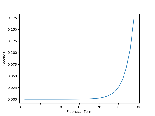
Observing that each call has two recursive calls we can place an upper bound on this function as O(2^n). However, if we solve this recurrence we can compute the exact value and place a tight bound for time complexity.
We can write a recurrence for the number of times fib is called:
T(1) = 1
T(n) = T(n-1) + T(n-2)
a^n = a^{n-1} + a^{n-2}
a^2 = a + 1
a = \frac{1 + sqrt(5)}{2}

T(n) = \frac{1 + sqrt(5)}{2}^n +  \frac{1 1 sqrt(5}{2}^n

O(1.618^n)
Measured Performance
Here is a graph of the actual performance that I observed for this algorithm.
Accumulation Solution
The problem with the previous recursive solution is that you had to recalculate certain terms of fibonacci a ton of times. A summation variable would help us avoid this problem. You could write this using a simple loop, however, it is still possible to do this with recursion.
def fibHelper(n, a, b):
    if n == 0:
        return a
    elif n == 1:
        return b
    return fibHelper(n-1, b, a+b)


def fibIterative(n):
    return fibHelper(n, 0, 1)
In this code example fibHelper is a method which accumulates the previous two terms. The fibIterative is a wrapper method which sets the two initial terms equal to 0 and 1 representing the fibonacci sequence.
Proof in latex that fibHelper
proof in latex that fib iterative = fib
Time Complexity
proof in latex for time complexity
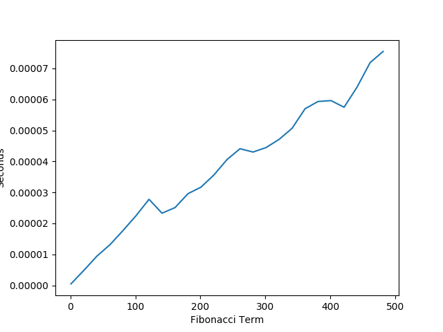
Measured Performance
Notice how much faster this solution is compared to the original recursive solution for Fibonacci. Also, I only measured going out to 500 because beyond that I hit the maximum number of recursive calls for my installation of Python.
Matrix Solution
We can actually get better than linear time for performance while calculating the Fibonacci sequence recursively.
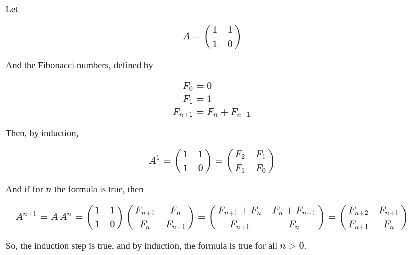
Without any other tricks, raising a matrix to a power n times would not get us better than linear performance. However, if we use the Exponentiation by Squaring method, we can expect to see logarithmic time.
def multiply(a,b):
    product = [0,0,0]
    product[0] = a[0]*b[0] + a[1]*b[1]
    product[1] = a[0]*b[1] + a[1]*b[2]
    product[2] = a[1]*b[1] + a[2]*b[2]
    return product


def power(l, k):
    if k == 1:
        return l
    temp = power(l, k//2)
    if k%2 == 0:
        return multiply(temp, temp)
    else:
        return multiply(l, multiply(temp, temp))


def fibPower(n):
    l = [1,1,0]
    return power(l, n)[1]
Time Complexity
latex proof for 9lg(n) performance
Measured Performance
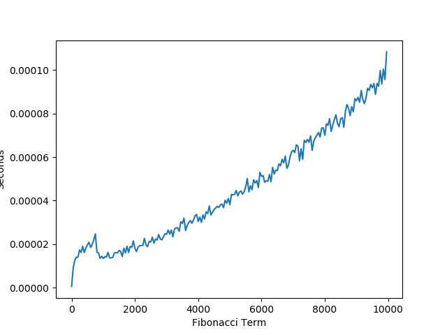
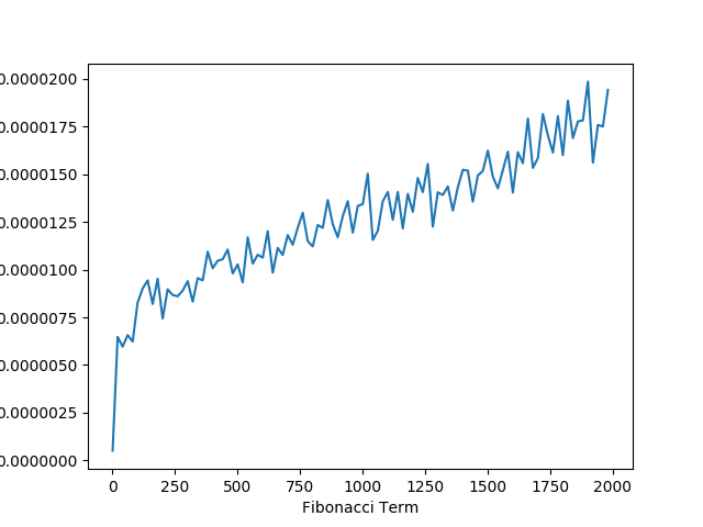 As expected by our mathmatical calcuations, the algorthem appears to be running in
logarithmic time.
Measured Performance With Large Numbers
When calculating the fibonacci term for extremely large numbers dispite having a polynomial time complexity, the space required to compute Fibonacci grows exponentially. Since our performance is only pseudo-polynomial we see a degrade in our performance when calculating large terms of the fibonacci sequence.
The one amazing thing to point out here is that despite calculating the 10,000 term of Fibonacci, this algorithm is nearly 400 times faster than the recursive algorithm when it was calculating the 30th term of Fibonacci.
Closed Form Definition
It is actually possible to calculate Fibonacci in constant time using a closed form definition.
latex proof of closed form definition

